Practical Data Modeling with dbt: Star vs. Snowflake Compared

Introduction

Data warehousing designs typically follow one of two popular schema patterns: star schema or snowflake schema. Both are dimensional modeling techniques used to organize data for analytics, but they differ in their approach to normalization. Let’s explore these concepts and see how they apply to modern analytics tools like dbt.

This guide is designed for data engineers and analytics engineers familiar with basic dbt usage, looking to understand practical schema modeling decisions in their analytics workflows.

Database Normalization vs. Denormalization

Before diving into these schemas, let’s understand the core concepts behind them.

Normalization is the process of organizing data to reduce redundancy by dividing large tables into smaller, related ones. This approach:

• Minimizes data duplication
• Ensures data integrity
• Makes updates more efficient (change data in only one place)
• Saves storage space

Denormalization is the opposite approach, deliberately introducing redundancy to optimize for read performance. This approach:

• Reduces the need for complex joins
• Speeds up query performance
• Simplifies query writing
• Optimizes for analytics workloads

Example of a Denormalized Table:

customer_id	customer_name	city	country
1	Alice	Paris	France
2	Bob	Paris	France
3	Charlie	London	UK

But suppose Paris changes its spelling (unlikely but imagine “Paris” becomes “París”). In the denormalized version, every customer row with Paris must be updated.
This increases the cost of updates (slow, error-prone) and risks inconsistencies (some rows updated, some not).

Normalization avoids this because the city name is stored once.

The Birth of Star Schema

Star schema emerged naturally from the need to optimize databases for analytical queries rather than transactional processing. In traditional OLTP (Online Transaction Processing) systems, normalization rules the day to ensure data integrity during frequent updates. However, data warehouses primarily serve read-heavy analytical workloads where query performance is prioritized over update efficiency.

A star schema consists of:

• A central fact table containing business measurements/metrics
• Multiple dimension tables surrounding the fact table like points of a star
• Simple keys connecting dimensions to facts

The Update Challenge in Star Schema

The denormalized nature of star schemas creates specific challenges when updates are needed:

1. Update Propagation: When dimension data changes, multiple records may need updating due to redundancy. For example, if a product category name changes, this update must be applied to all records containing that category.
2. Update Cost: The computational and time cost of updating denormalized data can be significant in large data warehouses.
3. Data Consistency: Partial updates can lead to inconsistent reporting if not properly managed.
4. Historical Tracking: Many star schemas use slowly changing dimensions (SCDs) to track historical changes, adding complexity.

However, these update challenges are generally accepted because data warehouses typically:

• Have scheduled batch updates rather than real-time changes
• Prioritize read performance over write performance
• Can rebuild dimensions from source systems when needed

Snowflake Schema: Taking Normalization Further

The snowflake schema evolved as an extension of the star schema, introducing normalization to the dimension tables. Instead of having completely denormalized dimension tables, snowflake schemas break dimensions into multiple related tables.

In a snowflake schema:

• The central fact table remains the same as in a star schema
• Dimension tables are normalized into multiple related dimension tables
• The resulting diagram resembles a snowflake with branching dimension tables

Advantages of Snowflake Schema:

• Reduced storage space through minimized redundancy
• Better data integrity due to normalization
• More efficient updates since data exists in one place
• Clearer representation of hierarchical relationships

Disadvantages of Snowflake Schema:

• More complex queries requiring additional joins
• Potentially slower query performance
• More difficult for business users to understand
• More complex ETL processes

Visualizing Star vs. Snowflake

This is an example of a star schema:

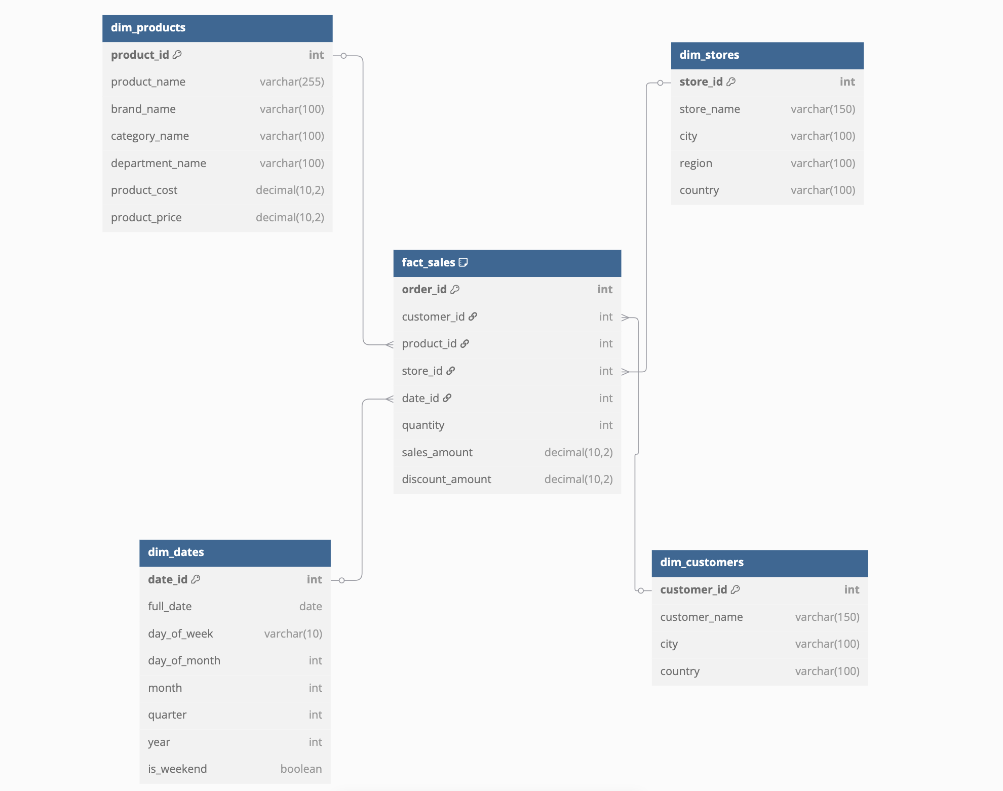
As you can see the fact_sales table is directly connected to dimensions tables.

Here is an example of a snowflake schema and as you can see there are more models, which increases complexity (as more joins are required to retrieve all the information that you would need)

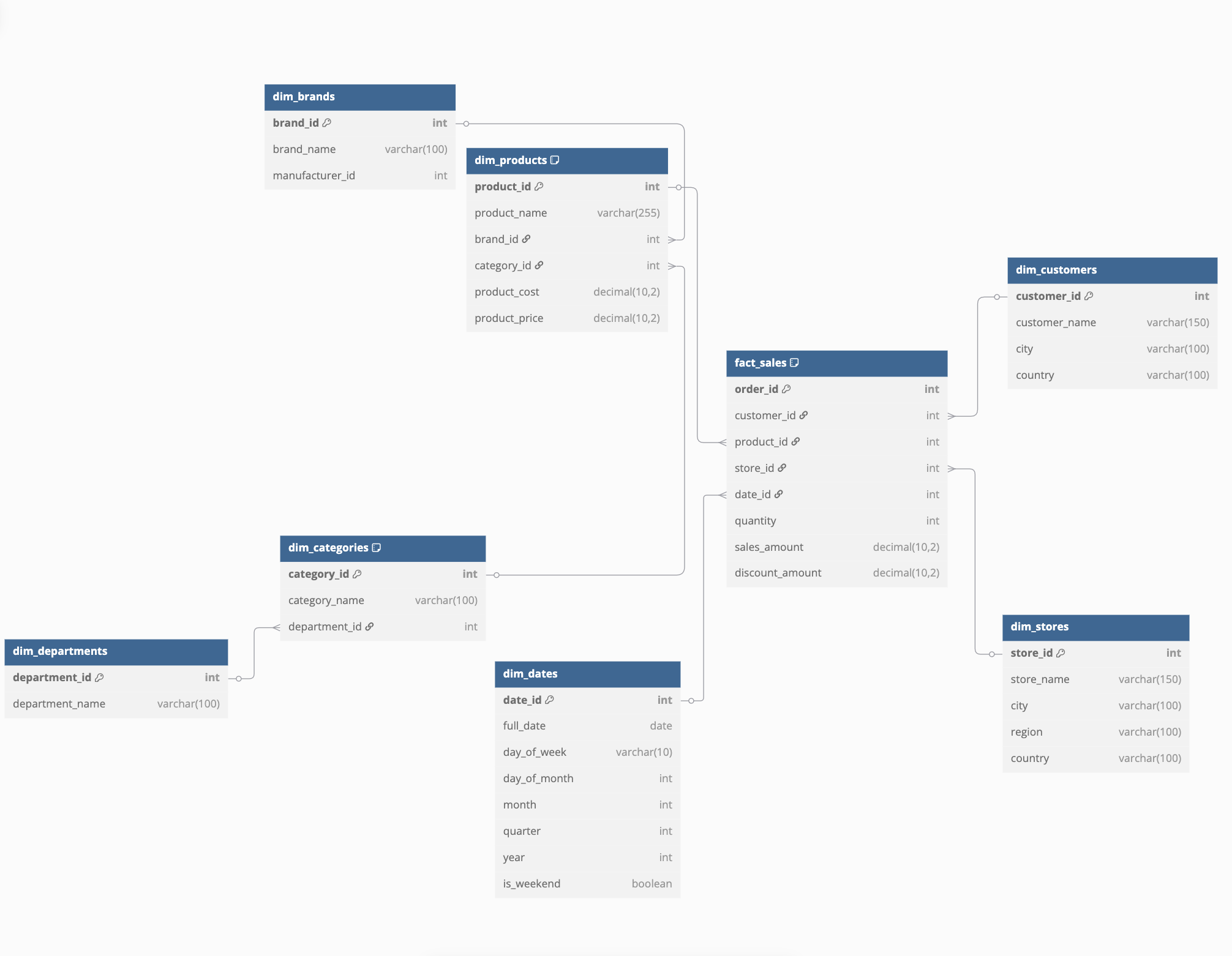
The fact_sales is connected to dimensions tables that are themselves connected to other dimensions tables.

Performance Considerations at Scale

The performance impact of each schema design varies based on several factors:

Query Pattern Impact

Star Schema:

• Excels at commonly used aggregation queries (e.g., “total sales by region”)
• Performs well with pre-defined dashboard queries
• Supports efficient slice-and-dice analytics with minimal joins

Snowflake Schema:

• Better suits queries that only need specific normalized dimension attributes
• May perform poorly on broad analytical queries requiring multiple dimension hops
• Requires more complex query optimization by the database engine

Data Volume Scaling

As data volumes grow into terabytes and beyond:

Star Schema:

• Maintains relatively consistent query performance as fact tables grow
• May face challenges with very large dimension tables
• Usually scales more predictably with modern columnar storage

Snowflake Schema:

• Can become increasingly complex to optimize at scale
• May experience exponential performance degradation with multi-level joins
• Often requires more careful indexing and query tuning

Modern Cloud Data Warehouse Optimizations

Different cloud data warehouses handle these schemas differently:

Data Warehouse	Star Schema Optimizations	Snowflake Schema Optimizations
Snowflake	Excellent caching of dimension tables; auto-clustering	Advanced join optimizations; good with multi-table normalized data
BigQuery	Strong columnar compression; broadcasts dimensions efficiently	Query optimizer that can rewrite some normalized queries
Redshift	Distribution keys on fact table foreign keys; sort keys on common filters	More reliant on proper distribution and sort key selection
Databricks	Delta Lake format optimizations; excellent for denormalized data	Can leverage query optimization for multi-hop joins

Practical Examples for dbt/BI Needs

Let’s illustrate both schemas using a retail analytics example:

Star Schema Example in dbt

• fact_sales:

-- models/mart/core/fact_sales.sql
select
  order_id,
  customer_id,
  product_id,
  store_id,
  date_id,
  quantity,
  sales_amount,
  discount_amount
from {{ ref('stg_sales') }}

• dim_products

-- models/marts/core/dim_products.sql
select
  product_id,
  product_name,
  brand_name,
  category_name,
  department_name,
  product_cost,
  product_price
from {{ ref('stg_products') }}

In dbt, you would model this as:

# dbt_project.yml schema configuration
models:
  retail_analytics:
    mart:
      core:
        - name: fact_sales
          description: "Sales fact table"
        - name: dim_products
          description: "Denormalized products dimension"
        - name: dim_customers
          description: "Customer dimension"
        - name: dim_stores
          description: "Store dimension"
        - name: dim_dates
          description: "Date dimension"

Snowflake Schema Example in dbt

The fact table would be identical to the one in the star schema.

• fact_sales

-- models/mart/core/fact_sales.sql
select
  order_id,
  customer_id,
  product_id,
  store_id,
  date_id,
  quantity,
  sales_amount,
  discount_amount
from {{ ref('stg_sales') }}

• dim_products

-- models/mart/core/dim_products.sql
select
  product_id,
  product_name,
  brand_id,
  category_id,
  product_cost,
  product_price
from {{ ref('stg_products') }}

• dim_brands

-- models/mart/core/dim_brands.sql
select
  brand_id,
  brand_name,
  manufacturer_id
from {{ ref('stg_brands') }}

• dim_category

-- models/mart/core/dim_categories.sql
select
  category_id,
  category_name,
  department_id
from {{ ref('stg_categories') }}

• dim_departments.sql

-- models/mart/core/dim_departments.sql
select
  department_id,
  department_name
from {{ ref('stg_departments') }}

In dbt, the snowflake schema would be modeled as:

# dbt_project.yml schema configuration
models:
  retail_analytics:
    mart:
      core:
        - name: fact_sales
          description: "Sales fact table"
        - name: dim_products
          description: "Products dimension"
        - name: dim_brands
          description: "Brand dimension" 
        - name: dim_categories
          description: "Product category dimension"
        - name: dim_departments
          description: "Department dimension"
        - name: dim_customers
          description: "Customer dimension"
        - name: dim_stores
          description: "Store dimension"
        - name: dim_dates
          description: "Date dimension"

As you can notice there are many more dimension tables and the dim_products contains information but is more connected to others models.

dbt Implementation Trade-offs

When implementing these schemas with dbt, several practical considerations come into play:

Materialization Strategies

Star Schema:

# Example dbt materialization for star schema
models:
  retail_analytics:
    mart:
      core:
        dim_products:
          materialized: table
          cluster_by: ['product_id']

• Tables: Often preferred for dimension tables due to their denormalized nature
• Incremental: Efficient for large fact tables, with clear unique keys
• Snapshots: Useful for tracking changes in dimensions (SCD Type 2)

Snowflake Schema:

# Example dbt materialization for snowflake schema
models:
  retail_analytics:
    mart:
      core:
        dim_categories:
          materialized: view  # For small, frequently changing dimensions
        dim_products:
          materialized: table
          cluster_by: ['product_id']

• Views: Can work well for smaller normalized dimension tables
• Mixed approach: Tables for large/frequently queried dimensions, views for others
• Ephemeral: Sometimes useful for intermediate normalized tables

Testing Strategies

Both schemas benefit from robust testing, but with different emphasis:

Star Schema Tests:

# Example tests for star schema
models:
  - name: dim_products
    columns:
      - name: product_id
        tests:
          - unique
          - not_null
      - name: product_name
        tests:
          - not_null
      - name: category_name  # Denormalized value needs consistency tests
        tests:
          - accepted_values:
              values: ["Electronics", "Apparel", "Home"]

• Focus on referential integrity between fact and dimension tables
• Validate denormalized values with custom tests
• Test for duplicates in denormalized dimensions

Snowflake Schema Tests:

# Example tests for snowflake schema relationships
models:
  - name: dim_products
    columns:
      - name: category_id
        tests:
          - relationships:
              to: ref('dim_categories')
              field: category_id
  - name: dim_categories
    columns:
      - name: category_name
        tests:
          - accepted_values:
              values: ["Electronics", "Apparel", "Home"]

• Focus more on testing relationships between normalized tables
• Test primary/foreign key relationships between dimension tables
• Centralize domain tests on the authoritative table for each attribute

Modern Data Stack Integration

The choice between star and snowflake schemas affects how your data interfaces with other components in the modern data stack:

Impact on BI Tools

Star Schema Benefits:

• Simpler for business users to understand and navigate
• Better performance with tools like Tableau, Power BI, and Looker
• Easier to create semantic layers and business-friendly naming

Snowflake Schema Challenges:

• May require more complex BI modeling to hide join complexity
• Can lead to slower dashboard performance without careful optimization
• May necessitate more maintenance of the semantic layer

Self-Service Analytics Capabilities

The schema choice significantly impacts how business users interact with data:

Star Schema:

-- Typical business user query with star schema
select 
    d.department_name,
    sum(f.sales_amount) as total_sales
from fact_sales f
join dim_products p on f.product_id = p.product_id
where p.department_name = 'Electronics'
group by d.department_name

Snowflake Schema:

-- Equivalent query with snowflake schema (more complex)
select 
  d.department_name, 
  sum(f.sales_amount) as total_sales
from fact_sales f
join dim_products p on f.product_id = p.product_id
join dim_categories c on p.category_id = c.category_id
join dim_departments d on c.department_id = d.department_id
where d.department_name = 'Electronics'
group by d.department_name

The snowflake schema query requires more understanding of the data model and creates more opportunities for incorrect joins.

Data Discovery and Documentation

Both schemas require thorough documentation in dbt, but with different emphasis:

# Star schema documentation focus
models:
  - name: dim_products
    description: "Complete product dimension with all attributes"
    columns:
      - name: product_id
        description: "Primary key for products"
      - name: category_name
        description: "Product category name"
      
# Snowflake schema documentation focus
models:
  - name: dim_products
    description: "Core product attributes"
    columns:
      - name: product_id
        description: "Primary key for products"
      - name: category_id
        description: "Foreign key to dim_categories"
  - name: dim_categories
    description: "Product categories"
    columns:
      - name: category_id
        description: "Primary key for categories"
      - name: category_name
        description: "Category name"

In the snowflake schema, thorough relationship documentation becomes even more critical.

Technical Considerations for Implementation

A few additional technical considerations can influence your schema choice:

Partitioning and Clustering Strategies

Star Schema:

• Partition fact tables by date/time dimensions
• Cluster dimension tables by primary keys
• Consider clustering fact tables by frequently filtered dimensions

# Example dbt configuration for star schema
models:
  - name: fact_sales
    config:
      materialized: incremental
      partition_by:
        field: date_id
        data_type: int
      cluster_by: ['product_id', 'store_id']

Snowflake Schema:

• Similar fact table strategies apply
• More complex analysis required to optimize multiple dimension hops
• May need to optimize for specific join paths

Incremental Loading Considerations

Both schemas present different challenges for incremental loading:

Star Schema:

-- Incremental load for star schema dimension
{{ config(
    materialized='incremental',
    unique_key='product_id'
) }}
 
select
    product_id,
    product_name,
    brand_name,
    category_name,
    -- More denormalized attributes
    current_timestamp() as updated_at
from source
{% if is_incremental() %}
    where updated_at > (select max(updated_at) from {{ this }})
{% endif %}

Snowflake Schema:

-- Need to handle multiple incremental models with dependencies
{{ config(
    materialized='incremental',
    unique_key='product_id'
) }}
 
select
    p.product_id,
    p.product_name,
    p.brand_id,
    p.category_id,
    current_timestamp() as updated_at
from source p
{% if is_incremental() %}
    where p.updated_at > (select max(updated_at) from {{ this }})
{% endif %}

The snowflake schema requires careful orchestration of incremental loads across related dimension tables to maintain referential integrity.

Data Pipeline Complexity

Star Schema Pipelines:

• Typically simpler overall architecture
• More complex transformation logic in each model
• More straightforward dependency graph

Snowflake Schema Pipelines:

• More complex overall architecture with more models
• Simpler transformation logic in each individual model
• More complex dependency graph requiring careful orchestration

Choosing Between Star and Snowflake for Modern BI

When deciding between star and snowflake schemas for your dbt or other BI implementations, consider:

1. Query Performance: Star schemas typically offer better performance for most analytical queries due to fewer joins.
2. Storage Considerations: Modern cloud data warehouses have made storage costs less important than they used to be.
3. Data Maintenance: If frequent dimension updates are required, snowflake schemas may be easier to maintain.
4. Business User Access: Star schemas are typically easier for business users to understand when writing their own queries.
5. Data Modeling Complexity: Complex hierarchical relationships may be more naturally represented in snowflake schemas.

Star Schema	Snowflake Schema
Faster queries	More normalized data
Easier for BI users	Better maintainability
More redundancy	Less redundancy
Good for simple reporting	Good for complex evolving data

Most modern data teams lean toward star schemas for their simplicity and performance benefits, especially with tools like dbt that make it easier to maintain the transformation logic required to denormalize data. Specifically, dbt’s modularity and ref() function simplify building and maintaining the necessary transformations for denormalized dimension tables in a star schema. However, hybrid approaches that selectively normalize only certain complex dimensions are also common, providing a balance between the two approaches. Even when snowflake structures are chosen for specific dimensions due to complexity or update frequency, dbt helps manage the increased join complexity by clearly defining model dependencies (ref()) and enabling robust testing and documentation of these multi-level relationships.

The choice ultimately depends on your specific analytical needs, query patterns, and how your team interacts with the data.